
External validation of a Cox prognostic model
Data preparation
First start by activating the survival package and do some data preparation.
library(survival)

df_dev <- survival::rotterdam # assign rotterdam data to development dataset
df_dev <- subset(df_dev, nodes>0) # select patients with positive nodes
df_dev$rfstime <- pmin(df_dev$rtime, df_dev$dtime) # determine outcome
df_dev$status  <- pmax(df_dev$recur, df_dev$death)

df_dev$rfstime <- df_dev$rfstime/365 # convert time to years
df_dev$status[df_dev$rfstime>=7] <- 0 # censor events after 7 years (84 months)

df_dev$rfstime[df_dev$rfstime>7] <- 7 # truncate survival time at 7 years

df_dev$size <- factor(df_dev$size) # define variables
df_dev$age <- df_dev$age/100
df_dev$er <- df_dev$er/1000
Methods
- Method 1: Regression on PI in validation data
- Method 2: Check model misspecification/fit
- Method 3: Measures of discrimination
- Method 4: Kaplan-Meier curves for risk groups
- Method 5: Logrank or Cox P-values
- Method 6: Hazard ratios between risk groups
- Method 7: Calibration and the baseline hazard function
Method 1: Regression on PI in validation data
Fit the model that was developed in the development dataset in the validation dataset to extract the predictor values.
fit_dev <-
  coxph(Surv(rfstime, status) ~ I(age^3) + I(age^3 * log(age)) + meno +
   factor(size) +  I((nodes)^-0.5) + er + hormon, data=df_dev) # fit model as in Table 2

library(sjPlot)
tab_model(fit_dev, transform=NULL, show.r2 = FALSE)| Surv(rfstime, status) | |||
|---|---|---|---|
| Predictors | Estimates | CI | p |
| I(age^3) | 1.14 | 0.36 – 1.92 | 0.004 |
| I(age^3 * log(age)) | 9.29 | 4.11 – 14.48 | <0.001 |
| pre/post meno | 0.46 | 0.22 – 0.71 | <0.001 |
| factor(size)20-50 | 0.24 | 0.09 – 0.40 | 0.002 |
| factor(size)>50 | 0.55 | 0.36 – 0.75 | <0.001 |
| I((nodes)^-0.5) | -1.70 | -1.98 – -1.42 | <0.001 |
| er | -0.32 | -0.58 – -0.06 | 0.015 |
| Hormonal therapy | -0.35 | -0.51 – -0.18 | <0.001 |
| Observations | 1546 | ||
From the description of the development and validation on Page 2 and 3, it is not possible to 100% replicate the results from the paper. As a consequence some results are different (but very close) from the results in the paper.
Next, define the PI of the development dataset in the validation dataset. Than center the PI in the validation dataset by using the same value to center the PI in the development dataset (page 5, under example). In our example that value is -1.290544 (in the paper that value is -1.32,
page 5, under example).
Xb_dev <- model.matrix(fit_dev) %*% coef(fit_dev)
Xbavg_dev <- sum(coef(fit_dev)*fit_dev$means)
PI_dev <- Xb_dev - Xbavg_dev # centered PI in development dataset (for discrimination later)
df_dev$PI_dev <- PI_dev

df_val <- survival::gbsg # validation data

df_val$size <- factor(cut(df_val$size, breaks = c(0, 20, 50, 125), labels = c(1,2,3)))
df_val$age <- df_val$age/100
df_val$er <- df_val$er/1000
df_val$rfstime <- df_val$rfstime/365 # convert to years

# fit model in validation data
fit_val <- coxph(Surv(rfstime, status) ~  I(age^3) + I(age^3*log(age)) + meno +
                   factor(size) +  I(nodes^-0.5) + er + hormon, data=df_val)

Xb_val <- model.matrix(fit_val) %*% coef(fit_dev) # determine Xb in validation data
                                                  # by using coefficients of development data
PI_val <- Xb_val - Xbavg_dev # center PI by using mean of PI of development data

df_val$PI_val <- PI_val

fit_val <- coxph(Surv(rfstime, status) ~ PI_val, data=df_val)
tab_model(fit_val, transform=NULL, show.r2 = FALSE)| Surv(rfstime, status) | |||
|---|---|---|---|
| Predictors | Estimates | CI | p |
| PI_val | 0.98 | 0.76 – 1.20 | <0.001 |
| Observations | 686 | ||
The PI in the validation dataset is 0.9833 (SE 0.11). In the paper this value is (0.97 (SE 0.11)).
fit_val_test <- coxph(Surv(rfstime, status) ~ PI_val + offset(PI_val), data=df_val)
tab_model(fit_val_test, transform=NULL, show.r2 = FALSE)| Surv(rfstime, status) | |||
|---|---|---|---|
| Predictors | Estimates | CI | p |
| PI_val | -0.02 | -0.24 – 0.20 | 0.881 |
| Observations | 686 | ||
The test if the slope deviates from one results in a p-value of (0.881) (Page 10, under Method 1 gives p-value of 0.8 or see for method Steyerberg, 2nd ed 15.3.3).
Back to Methods
Method 2: Check model misspecification/fit
Apply a Jointed test to evaluate if the regression coefficients from the derivation dataset differ when estimated in the validation dataset (page 7 under Check model misspecification/fit).
fit_val <- coxph(Surv(rfstime, status) ~ I(age^3) + I(age^3*log(age)) + meno +
            factor(size) +  I((nodes)^-0.5) + er + hormon + offset(PI_val), data=df_val)

round(2*(diff(fit_val$loglik)), 2) # Chi-squared value
## [1] 6.04round(1-pchisq(2*(diff(fit_val$loglik)), 8), 3) # p-value## [1] 0.643The Chi-sqaured value of the Likelihood Ratio test is 6.04 and the p-value 0.643. This means no lack of fit of the coefficients in the validation dataset (page 10, under Method 2, reported Chi-sqaured value is 6.08 and p-value 0.6)
Back to Methods
Method 3: Measures of discrimination
Calculate measures of discrimination in the derivation and validation dataset (page 9, Table 4).
# Derivation
library(rms)
library(survAUC)
rcorr.cens(-1*PI_dev, Surv(df_dev$rfstime, df_dev$status))[1] # Harrell's c-index
## C Index
## 0.6724282GHCI(PI_dev) # Gonen and Heller## [1] 0.6539831# Validation
rcorr.cens(-1*PI_val, Surv(df_val$rfstime, df_val$status))[1] # Harrell's c-index## C Index
## 0.6578093GHCI(df_val$PI_val) # Gonen and Heller## [1] 0.647129Back to Methods
Method 4: Kaplan-Meier curves for risk groups
Determine risk groups by categorizing the PI in four groups at the 16th, 50th and 84th centiles (page 5, under Example). Use the quantile function for that in the development and validation dataset. Create figure 2 on page 10.
# KM curve development data
quant_PI_dev <- quantile(PI_dev, probs=c(0, 0.16, 0.5, 0.84, 1)) # Determine risk groups
df_dev$Risk_group_dev <- cut(PI_dev, breaks = quant_PI_dev, include.lowest = TRUE,
                                 labels = c(1,2,3,4))
fit_dev <- survfit(Surv(rfstime, status) ~ Risk_group_dev, data = df_dev)
library(survminer)
p1 <- ggsurvplot(fit_dev) # survival curve in development dataset
p1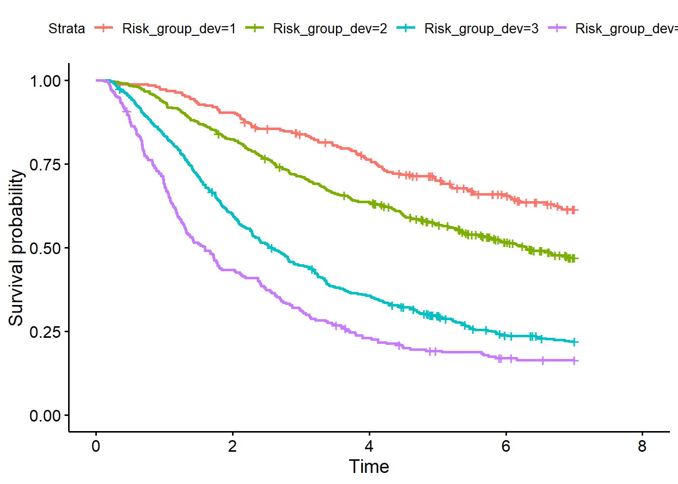
quant_PI_val <- quantile(PI_val, probs=c(0, 0.16, 0.5, 0.84, 1))
df_val$Risk_group_val <- cut(PI_val, breaks = quant_PI_val,
                                include.lowest = TRUE,  labels = c(1,2,3,4))

# KM curve validation data
fit_val <- survfit(Surv(rfstime, status) ~ Risk_group_val, data = df_val)
p2 <- ggsurvplot(fit_val) # survival curve in validation dataset

library(dplyr)
df_val_KM <- df_val %>%
  group_split(Risk_group_val)
surv_val <- lapply(df_val_KM, function(x){
  obj_surv <- survfit(Surv(rfstime, status) ~ 1, data = x)
  data.frame(time=obj_surv$time, surv=obj_surv$surv)
})

p1$plot +
  geom_step(data=surv_val[[1]], aes(x = time, y = surv), linetype=2) +
  geom_step(data=surv_val[[2]], aes(x = time, y = surv), linetype=2) +
  geom_step(data=surv_val[[3]], aes(x = time, y = surv), linetype=2) +
  geom_step(data=surv_val[[4]], aes(x = time, y = surv), linetype=2)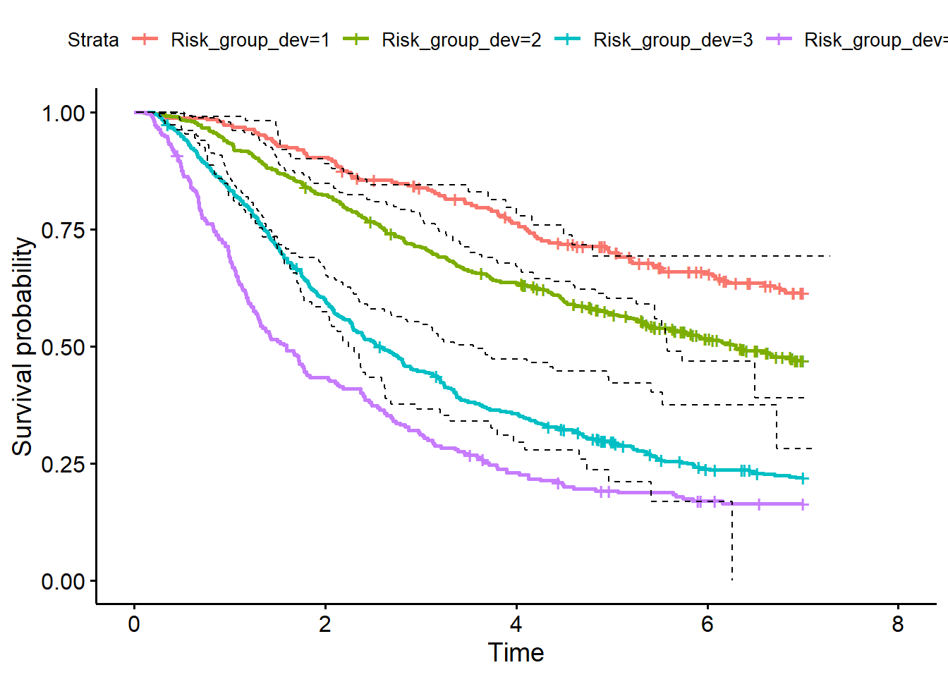
Back to Methods
Method 5: Logrank or Cox P-values
This method was deprecated in the paper. So no results are presented here.
Method 6: Hazard ratios between risk groups
These are comparable to those presented in Table 4 (page 9).
fit_dev_hr <- coxph(Surv(rfstime, status) ~ factor(Risk_group_dev), data=df_dev)
tab_model(fit_dev_hr, show.r2 = FALSE)| Surv(rfstime, status) | |||
|---|---|---|---|
| Predictors | Estimates | CI | p |
| Risk_group_dev [2] | 1.57 | 1.23 – 1.99 | <0.001 |
| Risk_group_dev [3] | 3.33 | 2.65 – 4.18 | <0.001 |
| Risk_group_dev [4] | 4.76 | 3.72 – 6.11 | <0.001 |
| Observations | 1546 | ||
fit_val_hr <- coxph(Surv(rfstime, status) ~ factor(Risk_group_val), data=df_val)
tab_model(fit_val_hr, show.r2 = FALSE)| Surv(rfstime, status) | |||
|---|---|---|---|
| Predictors | Estimates | CI | p |
| Risk_group_val [2] | 1.69 | 1.06 – 2.68 | 0.026 |
| Risk_group_val [3] | 3.14 | 2.01 – 4.92 | <0.001 |
| Risk_group_val [4] | 5.08 | 3.17 – 8.13 | <0.001 |
| Observations | 686 | ||
Back to Methods
Method 7: Calibration and the baseline hazard function
Start by modeling the baseline hazard function in the derivation data (Page 10, under Method 7 and continues on Page 11, and as result Figure 3).
# Fit the model in the derivation data
fit_dev <- coxph(Surv(rfstime, status) ~ I(age^3) + I(age^3 * log(age)) + meno +
                   factor(size) +  I((nodes)^-0.5) + er + hormon, data=df_dev)

bh <- basehaz(fit_dev) # Determine baseline hazard
baseh.all <- bh[match(df_dev$rfstime, bh[, 2]), 1] # match baseline hazard to all survival times
df_dev <- data.frame(df_dev, baseh.all)
# take log of baseline hazard and use as outcome for next step
df_dev$ln_bh <- log(df_dev$baseh.all)

# Model the log cumulative baseline hazard function (ln H0(t)) (Page 10, under Method 7)
fit_bh <- glm(ln_bh ~ I(rfstime^-0.5) +
                 I(rfstime^-0.5 * log(rfstime)) , data=df_dev)

tab_model(fit_bh, show.r2 = FALSE) # result of model fit| ln_bh | |||
|---|---|---|---|
| Predictors | Estimates | CI | p |
| (Intercept) | 1.74 | 1.73 – 1.76 | <0.001 |
| I(rfstime^-0.5) | -3.77 | -3.79 – -3.76 | <0.001 |
| I(rfstime^-0.5 * log(rfstime)) | -0.36 | -0.37 – -0.35 | <0.001 |
| Observations | 1546 | ||
log_H0_dev <- predict(fit_bh)
bh_pred <- exp(log_H0_dev)
gr <- factor(rep(1:2, each=1546), labels = c("Observed", "Predicted"))
df_plot <- data.frame(bh=c(df_dev$baseh.all, bh_pred), time=c(df_dev$rfstime, df_dev$rfstime), gr=gr)

p <- ggplot(df_plot, aes(x = time, y = bh, group=gr)) +
  geom_line(aes(color=gr)) + geom_rug(data = df_plot, aes(x = time), sides = "b")
p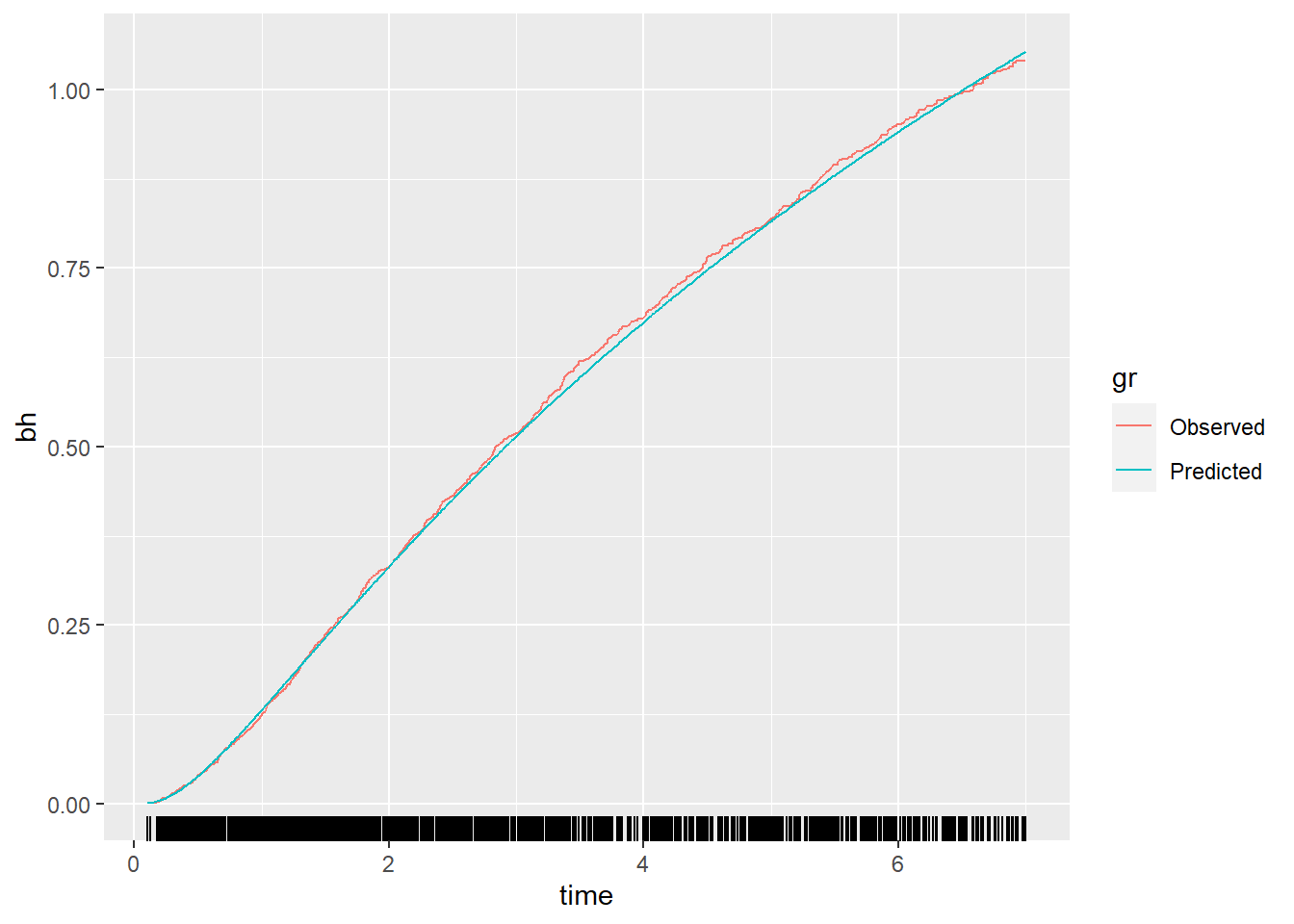
When the baseline hazard has been determined in the validation dataset continue with the calibration steps on Page 9, right column.
- Calculate S0(t) in the validation dataset
log_H0_val <- predict(fit_bh, newdata = df_val)
s0_val <- exp(-exp(log_H0_val)) # derive baseline survival function- For a given PI value compute the predicted survival function for each individual
pred_surv_val <- matrix(NA, nrow(df_val), nrow(df_val))
for(i in 1:nrow(df_val)){
  pred_surv_val[i, ] <- s0_val^exp(df_val$PI_val[i])
}
df_surv_val <- data.frame(LP_val=df_val$Risk_group_val, pred_surv_val)- Average the curves over all members of each risk group (add them to development dataset)
library(dplyr)
df_surv_mean_val <- df_surv_val %>%
  group_by(LP_val) %>%
  summarise_all("mean")

df_surv_mean_val <- t(df_surv_mean_val[, -1])
df_val <- data.frame(df_val, df_surv_mean_val)- Plot curves in validation data (Figure 4, page 11)
library(survminer)
fit<- survfit(Surv(rfstime, status) ~ Risk_group_val, data = df_val)
p1 <- ggsurvplot(fit)
p1$plot + geom_line(data=df_val, aes(x = rfstime, y = X1)) +
  geom_line(data=df_val, aes(x = rfstime, y = X2)) +
  geom_line(data=df_val, aes(x = rfstime, y = X3)) +
geom_line(data=df_val, aes(x = rfstime, y = X4)) 
In figure 4 also the predicted survival curves in the development dataset are added. So, also add them to the Figure by applying the same steps in the development dataset as in the validation data set.
# Step 1: determine So(t) in development dataset
s0_dev <- exp(-exp(log_H0_dev)) # derive baseline survival function

# Step 2: determine predicted survival function for each individual
pred_surv_dev <- matrix(NA, nrow(df_dev), nrow(df_dev))
for(i in 1:nrow(df_dev)){
  pred_surv_dev[i, ] <- s0_dev^exp(df_dev$PI_dev[i])
}
df_surv_dev <- data.frame(LP_dev=df_dev$Risk_group_dev, pred_surv_dev)

# Step 3: average the curves over all members of each risk group
library(dplyr)
df_surv_mean_dev <- df_surv_dev %>%
  group_by(LP_dev) %>%
  summarise_all("mean")

df_surv_mean_dev <- t(df_surv_mean_dev[, -1])
df_dev <- data.frame(df_dev, df_surv_mean_dev)

# Step 4: Plot curves
library(survminer)
fit<- survfit(Surv(rfstime, status) ~ Risk_group_val, data = df_val)
p1 <- ggsurvplot(fit)
p1$plot + geom_line(data=df_val, aes(x = rfstime, y = X1)) +
  geom_line(data=df_val, aes(x = rfstime, y = X2)) +
  geom_line(data=df_val, aes(x = rfstime, y = X3)) +
  geom_line(data=df_val, aes(x = rfstime, y = X4)) +
  geom_line(data=df_dev, aes(x = rfstime, y = X1), linetype=2) +
  geom_line(data=df_dev, aes(x = rfstime, y = X2), linetype=2) +
  geom_line(data=df_dev, aes(x = rfstime, y = X3), linetype=2) +
  geom_line(data=df_dev, aes(x = rfstime, y = X4), linetype=2)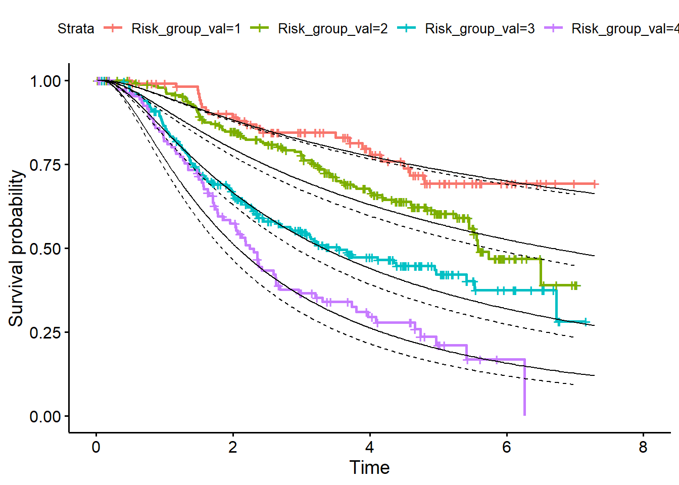
Back to Methods