
Prediction Modeling with the Cox model - all about the baseline hazard
Questions about the Cox model you were afraid to ask
Did you regularly ask yourself the following questions as, how is the baseline hazard function calculated and where can I use it for? What is the difference between centered=TRUE and centered=FALSE in the basehaz function? What is the result of the predict.coxph function and what is the difference between the options type=c("lp", "risk", "expected", "terms", "survival") in this function? What is the difference between predict.coxph and survfit? Where can I use the termplot function for and what is the difference between terms=1 and terms=2 in this function? These questions and more will be answered here!
How is the baseline hazard function calculated and where can I use it for?
The Cox model can be defined as follows,
\[ h(t) = h_0(t) \times exp(b_1x_1 + b_2x_2 + ... + b_px_p) \]
You could say that it consists of two separate parts, \(h_0(t)\) and \(exp(b_1x_1 + b_2x_2 + ... + b_px_p)\). The first part is called the baseline hazard function and the second part consists of the coefficients and predictor values (also called linear predictor, LP in short). If you know both of these parts you can produce the same results as the basehaz, survfit, predict.coxph and termplot functions and get a better understanding of what these functions do.
the Cox model can be applied in R using the coxph function. When you apply it you only get information about the \(exp(b_1x_1 + b_2x_2 + ... + b_px_p)\) part and not about the \(h_0(t)\) part as we will see when we fit a Cox model.
We generate a dataset with some example data that has no further meaning but is more used to compare results.
time <- c(1, 3, 5, 6, 2, 7, 9, 11)
status <- c(1, 0, 1, 1, 1, 0, 1, 1)
sex <- c(1, 1, 1, 1, 0, 0, 0, 0)
age <- c(57, 52, 48, 42, 39, 31, 26, 22)

df <- data.frame(time, status, sex, age)

fit_cox <- coxph(Surv(time, status) ~ age + sex, data=df, method = "breslow")
summary(fit_cox)
## Call:
## coxph(formula = Surv(time, status) ~ age + sex, data = df, method = "breslow")
##
## n= 8, number of events= 6
##
## coef exp(coef) se(coef) z Pr(>|z|)
## age 0.6338168 1.8847908 0.3917450 1.618 0.106
## sex -7.4935992 0.0005566 5.1135367 -1.465 0.143
##
## exp(coef) exp(-coef) lower .95 upper .95
## age 1.8847908 0.5306 8.746e-01 4.062
## sex 0.0005566 1796.5065 2.471e-08 12.538
##
## Concordance= 0.905 (se = 0.076 )
## Likelihood ratio test= 10.62 on 2 df, p=0.005
## Wald test = 2.72 on 2 df, p=0.3
## Score (logrank) test = 7 on 2 df, p=0.03Information about the the \(h_0(t)\) part is missing. However, this part is needed to produce e.g. predictions or generate survival curves. This can automatically be done with functions as survfit predict.coxph and termplot, but it is not always clear how they generate their results. That is exactly what this post will bring you hopefully, clarity about what these functions provide . To start from the beginning we will start with the basehaz function.
It all starts with the cumulative baseline hazard
When you look at the R Documentation file of the basehaz function (?basehaz) you can read that this function is an Alias for the survfit function (which means that either the basehaz or survfit function produce the same result. I will show that below) and you can read that basehaz produces the cumulative hazard (function).
The cumulative baseline hazard function can be calculated in two ways, when you apply an empty Cox model (or by using the observed data, i.e. no model), basehaz will give the same result as the Nelson-Aalen estimator and when we derive it from the Cox model including predictors basehaz will use the Breslow estimator.
I will show you how to calculate the cumulative baseline hazard manually for observed data and an empty Cox model and subsequently the Breslow estimator for a Cox model including predictors.
The Nelson-Aalen estimator
The formula for the Nelson-Aalen estimator is,
\[\widetilde{H}(t)= \sum_{t_i\le t}\frac{d_i}{n_i}\]
where \(d_i\) are the number of events of interest at time t, and \(n_i\) is the number of observations at risk. When we apply this formula manually we get,
time <- c(1,3,5,6, 2, 7, 9, 11)
status <- c(1, 0, 1, 1, 1, 0, 1, 1)
df <- data.frame(time, status)

df <- df[order(time), ] # order on time and events
d <- df$status
n <- length(d):1

H0 <- cumsum(d / n)
H0
## [1] 0.1250000 0.2678571 0.2678571 0.4678571 0.7178571 0.7178571 1.2178571
## [8] 2.2178571and the same result is provided by the basehaz function after we have fitted an empty Cox model.
time <- c(1,3,5,6, 2, 7, 9, 11)
status <- c(1, 0, 1, 1, 1, 0, 1, 1)

df <- data.frame(time, status)

fit_cox <- coxph(Surv(time, status) ~ 1 , data=df, method = "breslow")
basehaz(fit_cox)
## hazard time
## 1 0.1250000 1
## 2 0.2678571 2
## 3 0.2678571 3
## 4 0.4678571 5
## 5 0.7178571 6
## 6 0.7178571 7
## 7 1.2178571 9
## 8 2.2178571 11The Breslow estimator
The Breslow estimator for the baseline cumulative hazard is defined as (Hosmer and Lemeshow, 1999),
\[\widetilde{H_0}(t)=\sum_{t_i\leq t} \frac{d_i}{\sum e^{(X\beta)}}\] where \(d_i\) stands for the number of events of interest at time t and \(X\beta\) for the linear predictor scores (LP) .
When we apply this formula manually we get,
df <- data.frame(time, status, sex, age)

fit_cox <-
  coxph(Surv(time, status) ~ age + sex, x=TRUE, data=df, method = "breslow")

breslow_est <- function(time, status, X, B){
data <-
  data.frame(time, status, X)
data <-
  data[order(data$time), ]
t   <-
  unique(data$time)
k    <-
  length(t)
h    <-
  rep(0,k)

  for(i in 1:k) {
    lp <- (data.matrix(data[,-c(1:2)]) %*% B)[data$time>=t[i]]
    risk <- exp(lp)
    h[i] <- sum(data$status[data$time==t[i]]) / sum(risk)
  }

res <- cumsum(h)
return(res)
}
H0 <- breslow_est(time=df$time, status=df$status, X=fit_cox$x, B=fit_cox$coef)
H0
## [1] 3.442456e-13 5.942770e-12 5.942770e-12 1.096574e-10 1.897298e-09
## [6] 1.897298e-09 6.646862e-08 9.459174e-07This gives the same result as when the basehaz function is used after a Cox model is fitted and when we set centered=FALSE.
df <- data.frame(time, status, sex, age)

fit_cox <- coxph(Surv(time, status) ~ age + sex, data=df, method = "breslow")
basehaz(fit_cox, centered = FALSE)
## hazard time
## 1 3.442456e-13 1
## 2 5.942770e-12 2
## 3 5.942770e-12 3
## 4 1.096574e-10 5
## 5 1.897298e-09 6
## 6 1.897298e-09 7
## 7 6.646862e-08 9
## 8 9.459174e-07 11This is not a surprise, because the cumulative baseline hazard is calculated when the predictors are zero, i.e. when sex=0 and age=0 (more about this below under “When provide the basehaz and survfit functions the same results?”)
As a result of the basehaz function we get a dataframe with two columns, hazard and time. The column that is called hazard is the cumulative baseline hazard function \(H_0(t)\). Let’s take a closer look a the basehaz function.
What is the difference between centered=TRUE and centered=FALSE in basehaz?
We saw above that the manual version of the Breslow estimator and the basehaz function give the same results when centered=FALSE. When we choose for centered=TRUE the results are different. But of course we can make them equal. Than we have to mean center the linear predictor values.
If we look at the documentation of the basehazfunction under centered it says “if TRUE return data from a predicted survival curve at the mean values of the covariates fit$mean, if FALSE return a prediction for all covariates equal to zero”. Centering means that we calculate values against a sample reference value, and that reference value are the values we find under fit$mean.
df <- data.frame(time, status, sex, age)

fit_cox <- coxph(Surv(time, status) ~ age + sex, data=df, method = "breslow")
fit_cox$means
## age sex
## 39.625 0.000We see that the “means” are 39.625 and 0 respectively. Here we see that for the binary covariate sex, the reference value 0 is chosen. If we take a look at the R documentation for the coxph function and we look further at the documentation for the coxph.object (This class of objects is returned by the coxph class of functions to represent a fitted proportional hazards model) and look under means we find the following explanation vector of values used as the reference for each covariate and that is exactly what we get.
Mean centering the linear predictor values
Now we re-estimate the cumulative baseline hazard but now use the centered version of the linear predictor values, i.e. those calculated using fit$mean and subtracting these from the individual linear predictor values.
in formula form.
\[ LP_{sample} = \sum fit_{mean}*\beta's\] \[ LP_{indiv} = \sum X_i*\beta's\]
\[ LP_{centered} = LP_{indiv} - LP{sample}\]
To implement this we adjust the breslow_est function a little bit and include the LP_sample and LP_indiv objects that calculate the linear predictor values at the sample and individual values.
df <- data.frame(time, status, sex, age)

fit_cox <-
  coxph(Surv(time, status) ~ age + sex, x=TRUE, data=df, method = "breslow")

breslow_est_adj <- function(time, status, X, B){
data <-
  data.frame(time,status,X)
data <-
  data[order(data$time), ]
t   <-
  unique(data$time)
k    <-
  length(t)
h    <-
  rep(0,k)

  for(i in 1:k) {

    LP_sample <- sum(fit_cox$means * coef(fit_cox))
    LP_indiv <- c((0.6338168*(data$age)) + (-7.4935992*data$sex) )

    lp_centered <- (LP_indiv - LP_sample)[data$time>=t[i]]
    risk <- exp(lp_centered)
    h[i] <- sum(data$status[data$time==t[i]]) / sum(risk)
  }

res <- cumsum(h)
return(res)
}
H0 <- breslow_est_adj(time=df$time, status=df$status, X=fit_cox$x, B=fit_cox$coef)
H0
## [1] 2.780815e-02 4.800566e-01 4.800566e-01 8.858118e+00 1.532636e+02
## [6] 1.532636e+02 5.369326e+03 7.641106e+04Taking their difference is the same as using centered=TRUE in the basehaz function (the default).
When we apply that you can seethat we get the same result!
df <- data.frame(time, status, sex, age)

fit_cox <- coxph(Surv(time, status) ~ age + sex, data=df, method = "breslow")
basehaz(fit_cox, centered = TRUE)
## hazard time
## 1 2.780808e-02 1
## 2 4.800556e-01 2
## 3 4.800556e-01 3
## 4 8.858100e+00 5
## 5 1.532633e+02 6
## 6 1.532633e+02 7
## 7 5.369320e+03 9
## 8 7.641099e+04 11Mean centering the covariate values
In the Cox model centering is done to generate estimates against some kind of sample reference values (to represent some kind of reference population). For this the mean values of covariates are used as we have seen when we centered the linear predictor values. This seems a little bit awkward for categorical and binary variables like “sex” in our example. Sex represents male and female persons and taking the mean would say that we represent a population containing “average” sex persons. Therefore, for binary variables also the reference value of the binary variable is used and that is what is chosen for in the survival package. Mean centering the covariate values is the same as subtracting the mean of the covariate values from each person’s covariate value. When we do that we get the same result as mean centering the linear predictor values.
fit_cox <-
  coxph(Surv(time, status) ~ age + sex, x=TRUE, data=df, method = "breslow")

X_centered <- sweep(fit_cox$x, 2, fit_cox$means, "-")

H0 <- breslow_est(time=df$time, status=df$status, X=X_centered, B=fit_cox$coef)
H0
## [1] 2.780808e-02 4.800556e-01 4.800556e-01 8.858100e+00 1.532633e+02
## [6] 1.532633e+02 5.369320e+03 7.641099e+04When provide the basehaz and survfit functions the same results?
I have already mentioned that the basehaz function is an alias for the survfit function. That means that we can produce the same results for the cumulative baseline hazard function with the survfit function as with the basehaz function. Let’s explore that a little bit.
In the description of the centered term in the basehaz function it says if TRUE return data from a predicted survival curve at the mean values of the covariates fit$mean, if FALSE return a prediction for all covariates equal to zero. This latter means that we have to set all covariates to 0 in the survfit function to get the same results as the basehaz function with centered=FALSE. Let’s do that.
df <- data.frame(time, status, sex, age)

fit_cox <- coxph(Surv(time, status) ~ age + sex, data=df, method = "breslow")
fit_surv <- survfit(fit_cox, newdata = data.frame(age=0, sex=0))
fit_surv$cumhaz
## [1] 3.442456e-13 5.942770e-12 5.942770e-12 1.096574e-10 1.897298e-09
## [6] 1.897298e-09 6.646862e-08 9.459174e-07And that is indeed the case!
Now let’s see what we get when we use the default settings in the survfit function.
df <- data.frame(time, status, sex, age)

fit_cox <- coxph(Surv(time, status) ~ age + sex, data=df, method = "breslow")
fit_surv <- survfit(fit_cox)
fit_surv$cumhaz
## [1] 2.780808e-02 4.800556e-01 4.800556e-01 8.858100e+00 1.532633e+02
## [6] 1.532633e+02 5.369320e+03 7.641099e+04Now we see that We get the same result as the basehaz function with centered=TRUE. This means that as default the survfit function uses the mean centered variables with mean values that are stored under fit_cox$means.
We can check that when we give the values of the covariates to same value as under fit_cox$means.
df <- data.frame(time, status, sex, age)

fit_cox <- coxph(Surv(time, status) ~ age + sex, data=df, method = "breslow")
fit_surv <- survfit(fit_cox, newdata = data.frame(age=39.625, sex=0))
fit_surv$cumhaz
## [1] 2.780808e-02 4.800556e-01 4.800556e-01 8.858100e+00 1.532633e+02
## [6] 1.532633e+02 5.369320e+03 7.641099e+04We see that we indeed get the same results as for survfit(fit_cox) that we previously used!
The survfit function can not only be used to calculate the cumulative baseline hazard function, i.e. the cumulative hazard for a reference group, but also for other groups, depending on the values of the covariates. Eventually it can be used to produce survival curves for all kind of values for the covariates. I will show that later in another post.
What kind of results do we get with the predict.coxph function?
Now we now more about the cumulative baseline hazard function and the meaning of centering, it is easy to understand what kind of information the predict.coxph function generates.
See let’s take a closer look at this function and also in what way it provides results. In the predict.coxph function we can choose for the options type=c("lp", "risk", "expected", "terms", "survival"). What do they all mean?
type=“lp”
As default the predict.coxph function generates the “lp” values or linear predictor values.
df <- data.frame(time, status, sex, age)

fit_cox <- coxph(Surv(time, status) ~ age + sex, data=df, method = "breslow")
predict(fit_cox) # Same as predict(fit_cox, type="lp")
## [1] 3.5189684 0.3498842 -2.1853832 -5.9882842 -0.3961355 -5.4666703
## [7] -8.6357545 -11.1710219These are also stored under the fit_cox object and extracted by typing fit_cox$linear.predictors.
fit_cox$linear.predictors## [1] 3.5189684 0.3498842 -2.1853832 -5.9882842 -0.3961355 -5.4666703
## [7] -8.6357545 -11.1710219LP scores can also be calculated manually. We know now that the linear predictor of the Cox model is by default mean centered, i.e. calculated relative to the value of the sample mean (which was explained under **Mean centering the linear predictor values** above and also further explained in light of the predict.coxph function below under **What does it mean that predictions of type "risk" are relative to the sample**), so we have to apply that here also to get the correct LP values.
df <- data.frame(time, status, sex, age)

fit_cox <-
  coxph(Surv(time, status) ~ age + sex, x=TRUE, data=df, method = "breslow")

LP_indiv <- c((0.6338168*(df$age)) + (-7.4935992*df$sex) )

LP_sample <- c((0.6338168*(39.625)) + (-7.4935992*0) )
LP_sample
## [1] 25.11499LP <- LP_indiv - LP_sample
LP## [1] 3.5189677 0.3498837 -2.1853835 -5.9882843 -0.3961355 -5.4666699
## [7] -8.6357539 -11.1710211The same result is obtained by using the reference option in the predict.coxph function
predict(fit_cox, reference="sample")## [1] 3.5189684 0.3498842 -2.1853832 -5.9882842 -0.3961355 -5.4666703
## [7] -8.6357545 -11.1710219And this again is the same as mean centering the covariate values and subsequently calculating the linear predictor values.
df <- data.frame(time, status, sex, age)

LP <- c((0.6338168*(df$age-39.625)) + (-7.4935992*df$sex) )
LP
## [1] 3.5189677 0.3498837 -2.1853835 -5.9882843 -0.3961355 -5.4666699
## [7] -8.6357539 -11.1710211Now we know that the predict.coxph function uses as default a mean centered linear predictor.
What does it mean that predictions of type “risk” are relative to the sample
If we look at the R documentation of the predict.coxph function we find under details the following explanation: “The Cox model is a relative risk model; predictions of type”linear predictor”, “risk”, and “terms” are all relative to the sample from which they came. By default, the reference value for each of these is the mean covariate within strata.”
Let’s see what this means for the calculation of the LP scores. We first calculate the LP scores by using the mean of the covariates (mean of 39.625 for age and the reference value of 0 for sex):
df <- data.frame(time, status, sex, age)

fit_cox <-
  coxph(Surv(time, status) ~ age + sex, x=TRUE, data=df, method = "breslow")

LP_sample <- c((0.6338168*(39.625)) + (-7.4935992*0))
LP_sample
## [1] 25.11499Than we calculate the LP scores for all individuals in our dataset.
df <- data.frame(time, status, sex, age)

fit_cox <-
  coxph(Surv(time, status) ~ age + sex, x=TRUE, data=df, method = "breslow")

LP_indiv <- c((0.6338168*(df$age)) + (-7.4935992*df$sex) )
LP_indiv
## [1] 28.63396 25.46487 22.92961 19.12671 24.71886 19.64832 16.47924 13.94397Than we subtract the LP score at the mean of the sample (mean of the covariates) from the LP scores of the persons in our sample and exponentiate these values.
exp(LP_indiv - LP_sample)## [1] 3.374957e+01 1.418903e+00 1.124346e-01 2.507963e-03 6.729155e-01
## [6] 4.225279e-03 1.776396e-04 1.407626e-05We than get the same results as the “risk” results, but now see more clear that the LP and risk scores are calculated against the mean values of the covariates in the sample.
type=“risk
When we use this option hazard ratio’s are calculated with as the reference value the LP scores at the means of the covariates.
df <- data.frame(time, status, sex, age)

fit_cox <- coxph(Surv(time, status) ~ age + sex, data=df, method = "breslow")
predict(fit_cox, type="risk")
## [1] 3.374960e+01 1.418903e+00 1.124346e-01 2.507963e-03 6.729155e-01
## [6] 4.225278e-03 1.776395e-04 1.407625e-05The function will therefore produce the same results when we exponentiate the LP values.
df <- data.frame(time, status, sex, age)

fit_cox <-
  coxph(Surv(time, status) ~ age + sex, x=TRUE, data=df, method = "breslow")

LP_indiv <- c((0.6338168*(df$age)) + (-7.4935992*df$sex) )

LP_sample <- c((0.6338168*(39.625)) + (-7.4935992*0) )
LP_sample
## [1] 25.11499LP <- LP_indiv - LP_sample
risk <- exp(LP)
risk## [1] 3.374957e+01 1.418903e+00 1.124346e-01 2.507963e-03 6.729155e-01
## [6] 4.225279e-03 1.776396e-04 1.407626e-05type=“expected”
When we use this option we get the following results.
df <- data.frame(time, status, sex, age)

fit_cox <- coxph(Surv(time, status) ~ age + sex, data=df, method = "breslow")
predict(fit_cox, type="expected")
## 1 2 3 4 5 6 7 8
## 0.9385114 0.6811525 0.9959573 0.3843788 0.3230369 0.6475801 0.9538031 1.0755799In the R documentation is described that: “Predictions of type”expected” incorporate the baseline hazard and are thus absolute instead of relative”.
For these predictions we need the cumulative baseline hazard function, which we can easily obtain by the basehaz function. To get the same result as the predict.coxph function we first use the default settings of the basehaz function, i.e. centered=TRUE and than multiply these values with the (default) (mean centered) linear predictor values.
df <- data.frame(time, status, sex, age)

fit_cox <- coxph(Surv(time, status) ~ age + sex, data=df, method = "breslow")
H0 <- basehaz(fit_cox)
LP <- predict(fit_cox, type="lp")

H0[, 1]*exp(LP)
## [1] 0.93851138 0.68115250 0.05397488 0.02221579 103.13326837
## [6] 0.64758014 0.95380312 1.07557986type=“terms”
When we use this option we get the following values. These are the linear predictor values for each covariate (term) separately.
df <- data.frame(time, status, sex, age)

fit_cox <- coxph(Surv(time, status) ~ age + sex, data=df, method = "breslow")
predict(fit_cox, type="terms")
## age sex
## 1 11.0125677 -7.493599
## 2 7.8434834 -7.493599
## 3 5.3082161 -7.493599
## 4 1.5053150 -7.493599
## 5 -0.3961355 0.000000
## 6 -5.4666703 0.000000
## 7 -8.6357545 0.000000
## 8 -11.1710219 0.000000
## attr(,"constant")
## [1] 25.11499The information under attr(,"constant") is the linear predictor value of the reference population. As default value type="terms" provides the linear predictor values of all terms (covariates) in the model. With terms it is possible to get the linear predictor values for each separate covariate in the model.
df <- data.frame(time, status, sex, age)

fit_cox <- coxph(Surv(time, status) ~ age + sex, data=df, method = "breslow")
predict(fit_cox, type="terms", terms = "age") # same as terms = 1
## age
## 1 11.0125677
## 2 7.8434834
## 3 5.3082161
## 4 1.5053150
## 5 -0.3961355
## 6 -5.4666703
## 7 -8.6357545
## 8 -11.1710219
## attr(,"constant")
## [1] 25.11499These linear predictor values are calculated as,
LP_age <- 0.6338168*df$age - (0.6338168*39.625)
LP_age
## [1] 11.0125669 7.8434829 5.3082157 1.5053149 -0.3961355 -5.4666699
## [7] -8.6357539 -11.1710211and for the covariate sex,
df <- data.frame(time, status, sex, age)

fit_cox <- coxph(Surv(time, status) ~ age + sex, data=df, method = "breslow")
predict(fit_cox, type="terms", terms = "sex") # same as terms = 2
## sex
## 1 -7.493599
## 2 -7.493599
## 3 -7.493599
## 4 -7.493599
## 5 0.000000
## 6 0.000000
## 7 0.000000
## 8 0.000000
## attr(,"constant")
## [1] 25.11499These linear predictor values are calculated as.
LP_age <- -7.4935992*df$sex - (-7.4935992*0)
LP_age
## [1] -7.493599 -7.493599 -7.493599 -7.493599 0.000000 0.000000 0.000000
## [8] 0.000000So, each covariate uses it’s own reference value.
type=“survival”
This option is used to calculate survival probabilities.
df <- data.frame(time, status, sex, age)

fit_cox <- coxph(Surv(time, status) ~ age + sex, data=df, method = "breslow")
predict(fit_cox, type="survival")
## 1 2 3 4 5 6 7 8
## 0.3912098 0.5060335 0.3693697 0.6808734 0.7239472 0.5233106 0.3852730 0.3410999Using the cumulative hazard to calculate survival probabilities we can make use of the following formula,
\[S(t) = exp(-H(t)\]
We have seen under **type="expected"** how to calculate the cumulative hazard values. We can make use of the same calculations and include these in the formula for the survival probability.
df <- data.frame(time, status, sex, age)

fit_cox <- coxph(Surv(time, status) ~ age + sex, data=df, method = "breslow")
H0 <- basehaz(fit_cox)
LP <- predict(fit_cox, type="lp")

exp(-H0[, 1]*exp(LP))
## [1] 3.912098e-01 5.060335e-01 9.474559e-01 9.780292e-01 1.621028e-45
## [6] 5.233106e-01 3.852730e-01 3.410999e-01This is of course the same as,
df <- data.frame(time, status, sex, age)

fit_cox <- coxph(Surv(time, status) ~ age + sex, data=df, method = "breslow")
exp(-predict(fit_cox, type="expected"))
## 1 2 3 4 5 6 7 8
## 0.3912098 0.5060335 0.3693697 0.6808734 0.7239472 0.5233106 0.3852730 0.3410999Where can we use the termplot function for?
If we take a look at the R documentation of the termplot function we can read that with this function it is possible to plot regression terms. We can further read that we can extract the information that is plotted when we set plot=FALSE.
df <- data.frame(time, status, sex, age)

fit_cox <- coxph(Surv(time, status) ~ age + sex, data=df, method = "breslow")
termplot(fit_cox, plot=FALSE)
## $age
## x y
## 1 22 -11.1710219
## 2 26 -8.6357545
## 3 31 -5.4666703
## 4 39 -0.3961355
## 5 42 1.5053150
## 6 48 5.3082161
## 7 52 7.8434834
## 8 57 11.0125677
##
## $sex
## x y
## 1 0 0.000000
## 2 1 -7.493599
##
## attr(,"constant")
## [1] 25.11499We see that we get the same information as that is provided by the predict.coxph function and than option type="terms". The values that are provided are the linear predictor values related to each covariate. For continuous predictors the ordered unique values are provided and for a factor the values related to each category (level).
There is also the possibility to choose for specific covariate (term) values as was possible with the predict.coxph function.
df <- data.frame(time, status, sex, age)

fit_cox <- coxph(Surv(time, status) ~ age + sex, data=df, method = "breslow")
termplot(fit_cox, plot=FALSE, terms="age")
## $age
## x y
## 1 22 -11.1710219
## 2 26 -8.6357545
## 3 31 -5.4666703
## 4 39 -0.3961355
## 5 42 1.5053150
## 6 48 5.3082161
## 7 52 7.8434834
## 8 57 11.0125677
##
## attr(,"constant")
## [1] 25.11499To make a plot of the linear predictor values we can set plot=TRUE (default).
df <- data.frame(time, status, sex, age)

fit_cox <- coxph(Surv(time, status) ~ age + sex, data=df, method = "breslow")
termplot(fit_cox, plot=TRUE, terms="age")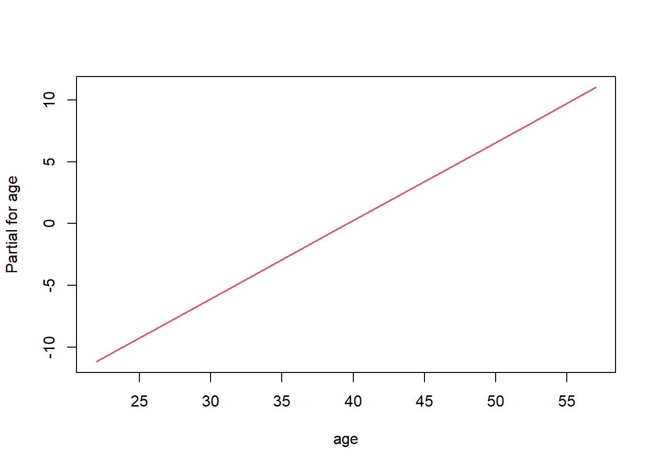
This is especially informative if the model would include non-linear or spline terms.
From hazard to survival
What we all can do with these functions in terms of survival probabilities and survival curves will be explained in another post (probably published in February 2023).
References
Hosmer, D.W. and Lemeshow, S. (1999) Applied Survival Analysis, Regression Modeling of Time to Event Data. John Wiley and Sons, New York.
Klein, J.P. and Moeschberger, S. (2003) Survival Analysis: Techniques for Censored and Truncated Data. 2nd edition. Springer, Berlin.
Moore, D.F. (2016) Applied Survival Analysis Using R. Use R. Springer, Berlin.