
Steps to externally validate a prediction model
Prediction model
We will externally validate the following prediction model:
library(foreign)
dat.orig <- read.spss(file="Hipstudy.sav", to.data.frame=TRUE)

library(rms)
dd <- datadist(dat.orig)
options(datadist='dd')

dat.orig$Mobility <- factor(dat.orig$Mobility)
fit.orig <- lrm(Mortality ~ Gender + Mobility + Age + ASA, x = T, y = T, data = dat.orig)
fit.orig
## Logistic Regression Model
##
## lrm(formula = Mortality ~ Gender + Mobility + Age + ASA, data = dat.orig,
## x = T, y = T)
##
## Model Likelihood Discrimination Rank Discrim.
## Ratio Test Indexes Indexes
## Obs 426 LR chi2 70.28 R2 0.234 C 0.774
## 0 333 d.f. 5 R2(5,426)0.142 Dxy 0.548
## 1 93 Pr(> chi2) <0.0001 R2(5,218.1)0.259 gamma 0.550
## max |deriv| 1e-06 Brier 0.145 tau-a 0.187
##
## Coef S.E. Wald Z Pr(>|Z|)
## Intercept -9.2172 1.6059 -5.74 <0.0001
## Gender 0.4623 0.2968 1.56 0.1194
## Mobility=2 0.4999 0.3014 1.66 0.0971
## Mobility=3 1.8148 0.5723 3.17 0.0015
## Age 0.0711 0.0189 3.75 0.0002
## ASA 0.7219 0.2144 3.37 0.0008
## pred.orig <- predict(fit.orig, type="fitted")ROC curve and AUC
library(pROC)
roc(fit.orig$y, pred.orig, ci=TRUE, plot = TRUE)
## Setting levels: control = 0, case = 1## Setting direction: controls < cases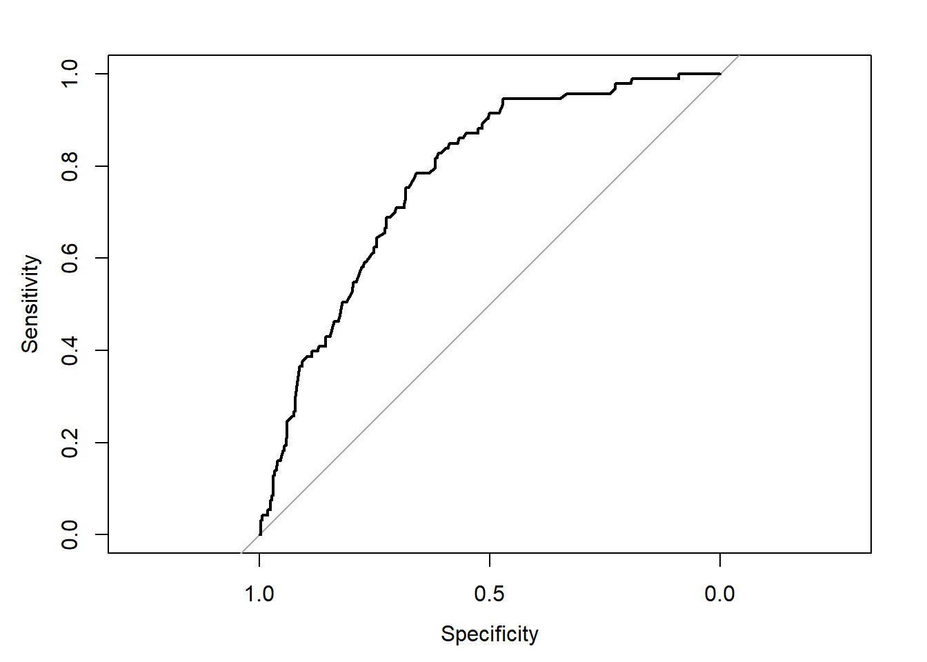
##
## Call:
## roc.default(response = fit.orig$y, predictor = pred.orig, ci = TRUE,     plot = TRUE)
##
## Data: pred.orig in 333 controls (fit.orig$y 0) < 93 cases (fit.orig$y 1).
## Area under the curve: 0.7738
## 95% CI: 0.7244-0.8232 (DeLong)
Calibration curve and H&L test
group.cut <- quantile(pred.orig, c(seq(0, 1, 0.1)))
group <- cut(pred.orig, group.cut)
pred.prob <- tapply(pred.orig, group, mean)

# Observed probabilities
obs.prob <- tapply(fit.orig$y, group, mean)
cal.m <- data.frame(cbind(pred.prob, obs.prob))
library(ggplot2)
plot(ggplot(cal.m,aes(x=pred.prob,y=obs.prob)) +
scale_x_continuous(name = "Predicted Probabilities",
breaks = seq(0, 1, 0.1), limits=c(0, 0.8)) +
scale_y_continuous(name = "Observed Probabilities",
breaks = seq(0, 1, 0.1), limits=c(0, 0.8)) +
geom_smooth(method='lm', formula = y~x, se = FALSE) +
geom_point(size=2, shape = 19) +
geom_abline(intercept = 0, slope = 1, linetype=2) +
ggtitle("Calibration Curve") )
library(ResourceSelection)
hoslem.test(fit.orig$y, pred.orig) # Hosmer and Lemeshow test from package ResourceSelection
##
## Hosmer and Lemeshow goodness of fit (GOF) test
##
## data: fit.orig$y, pred.orig
## X-squared = 4.6762, df = 8, p-value = 0.7916This model has an C-index (ROC) value of 0.774 and an R2 of 0.234. The Hosmer and Lemeshow test is not significant (for now we use it as a quick test) indicating that the model calibrates well.
Steps to externally validate a prediction model
1. Determine the Linear Predictor of the model. This is in our case:
coef.orig <- coef(fit.orig)
coef.orig # Coefficients of original model
## Intercept Gender Mobility=2 Mobility=3 Age ASA
## -9.21721717 0.46226952 0.49991610 1.81481732 0.07109868 0.721888612. Transport the original regression coefficients to the external dataset and calculate the linear predictor.
fit.ext <- lrm(Mortality ~ Gender + Mobility + Age + ASA, x = T, y = T, data = dat.ext)
lp.ext <- model.matrix(fit.ext) %*% coef.orig # model.matrix extracts predictor values of external dataset, including dummy coded variables.

# The same as above. Use for newdata the external dataset
lp.ext <- predict(fit.orig, newdata=dat.ext)
3. Determine the amount of miscalibration in intercept and calibration slope.
fit.ext.lp <- lrm(fit.ext$y ~ lp.ext)
fit.ext.lp
## Logistic Regression Model
##
## lrm(formula = fit.ext$y ~ lp.ext)
##
## Model Likelihood Discrimination Rank Discrim.
## Ratio Test Indexes Indexes
## Obs 300 LR chi2 43.89 R2 0.205 C 0.750
## 0 230 d.f. 1 R2(1,300)0.133 Dxy 0.499
## 1 70 Pr(> chi2) <0.0001 R2(1,161)0.234 gamma 0.501
## max |deriv| 2e-10 Brier 0.156 tau-a 0.179
##
## Coef S.E. Wald Z Pr(>|Z|)
## Intercept -0.6594 0.1567 -4.21 <0.0001
## lp.ext 0.8767 0.1554 5.64 <0.0001
## The coefficient values of -0.6594 and 0.8767 for the intercept and slope respectively indicate the amount of miscalibration in the intercept ansd slope value. Without miscalibration these values are 0 and 1 respectively.
4. Deterimne Discrimination and Calibration in the external dataset
Discrimination
pred.ext <-  1/(1+exp(-lp.ext))

roc(fit.ext$y, pred.ext, ci=TRUE, plot = TRUE)
## Setting levels: control = 0, case = 1## Setting direction: controls < cases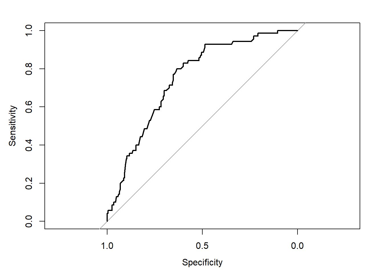
##
## Call:
## roc.default(response = fit.ext$y, predictor = pred.ext, ci = TRUE,     plot = TRUE)
##
## Data: pred.ext in 230 controls (fit.ext$y 0) < 70 cases (fit.ext$y 1).
## Area under the curve: 0.7496
## 95% CI: 0.6893-0.8098 (DeLong)
The AUC drops from 0.774 to 0.7496.
Calibration
# Predicted probabilities
pred.ext <-  1/(1+exp(-lp.ext))
group.cut <- quantile(pred.ext, c(seq(0, 1, 0.1)))
group <- cut(pred.ext, group.cut)
pred.prob <- tapply(pred.ext, group, mean)

# Observed probabilities
obs.prob <- tapply(fit.ext$y, group, mean)
cal.m.ext <- data.frame(cbind(pred.prob, obs.prob))
library(ggplot2)
plot(ggplot(cal.m.ext,aes(x=pred.prob,y=obs.prob)) +
scale_x_continuous(name = "Predicted Probabilities",
breaks = seq(0, 1, 0.1), limits=c(0, 0.8)) +
scale_y_continuous(name = "Observed Probabilities",
breaks = seq(0, 1, 0.1), limits=c(0, 0.8)) +
geom_smooth(method="lm", formula = y~x, se = FALSE) +
geom_point(size=2, shape = 19) +
geom_abline(intercept = 0, slope = 1, linetype=2) +
ggtitle("Calibration Curve") )
The calibration curve deviates from the ideal line.
Hosmer and Lemeshow test
hoslem.test(fit.ext$y, pred.ext)##
## Hosmer and Lemeshow goodness of fit (GOF) test
##
## data: fit.ext$y, pred.ext
## X-squared = 23.991, df = 8, p-value = 0.0023The Hosmer and Lemeshow test is now significant. The test confirms the miscalibration in the intercept and calibration slope, visualized on the calibration curve.
Incorrect external validation: recalibrated predictions
When you externally validate a prediction model you have to use
uncalibrated predictions. Otherwise the external validation
procedure is incorrect.
The correct uncalibrated predictions were used in the calibration curve above and were calculated “outside” the model to detect miscalibration by using the following formula to calculate predicted probabilities:
pred.ext <- 1/(1+exp(-lp.ext))Incorrect Calibrated predictions are calculated via the prediction model, when you use:
fit.ext.lp <- lrm(fit.ext$y ~ lp.ext) # the coefficient values reflect the amount of miscalibration
fit.ext.lp
## Logistic Regression Model
##
## lrm(formula = fit.ext$y ~ lp.ext)
##
## Model Likelihood Discrimination Rank Discrim.
## Ratio Test Indexes Indexes
## Obs 300 LR chi2 43.89 R2 0.205 C 0.750
## 0 230 d.f. 1 R2(1,300)0.133 Dxy 0.499
## 1 70 Pr(> chi2) <0.0001 R2(1,161)0.234 gamma 0.501
## max |deriv| 2e-10 Brier 0.156 tau-a 0.179
##
## Coef S.E. Wald Z Pr(>|Z|)
## Intercept -0.6594 0.1567 -4.21 <0.0001
## lp.ext 0.8767 0.1554 5.64 <0.0001
## pred.ext.recal <- predict(fit.ext.lp, type="fitted")These predictions are calibrated in the model by using the intercept and slope coefficient values as correction factors. These values are -0.6594 and 0.8631 for the intercept and slope respectively (equal to the values of step 3). Without miscalibration these intercept and slope coefficient values would be 0 and 1. These recalibrated predictions lead to the following results for discrimination and calibration.
Discrimination
roc(fit.ext$y, pred.ext.recal, ci=TRUE, plot = TRUE)## Setting levels: control = 0, case = 1## Setting direction: controls < cases
##
## Call:
## roc.default(response = fit.ext$y, predictor = pred.ext.recal,     ci = TRUE, plot = TRUE)
##
## Data: pred.ext.recal in 230 controls (fit.ext$y 0) < 70 cases (fit.ext$y 1).
## Area under the curve: 0.7496
## 95% CI: 0.6893-0.8098 (DeLong)
Calibration
library(ggplot2)
cal.plot <- ggplot(cal.m.ext,aes(x=pred.prob,y=obs.prob)) +
  scale_x_continuous(name = "Predicted Probabilities",
    breaks = seq(0, 1, 0.1), limits=c(0, 0.8)) +
  scale_y_continuous(name = "Observed Probabilities",
    breaks = seq(0, 1, 0.1), limits=c(0, 0.8)) +
  geom_smooth(method="lm", formula = y~x, se = FALSE) +
  geom_point(size=2, shape = 19) +
  geom_abline(intercept = 0, slope = 1, linetype=2) +
  ggtitle("Calibration Curve")
plot(cal.plot)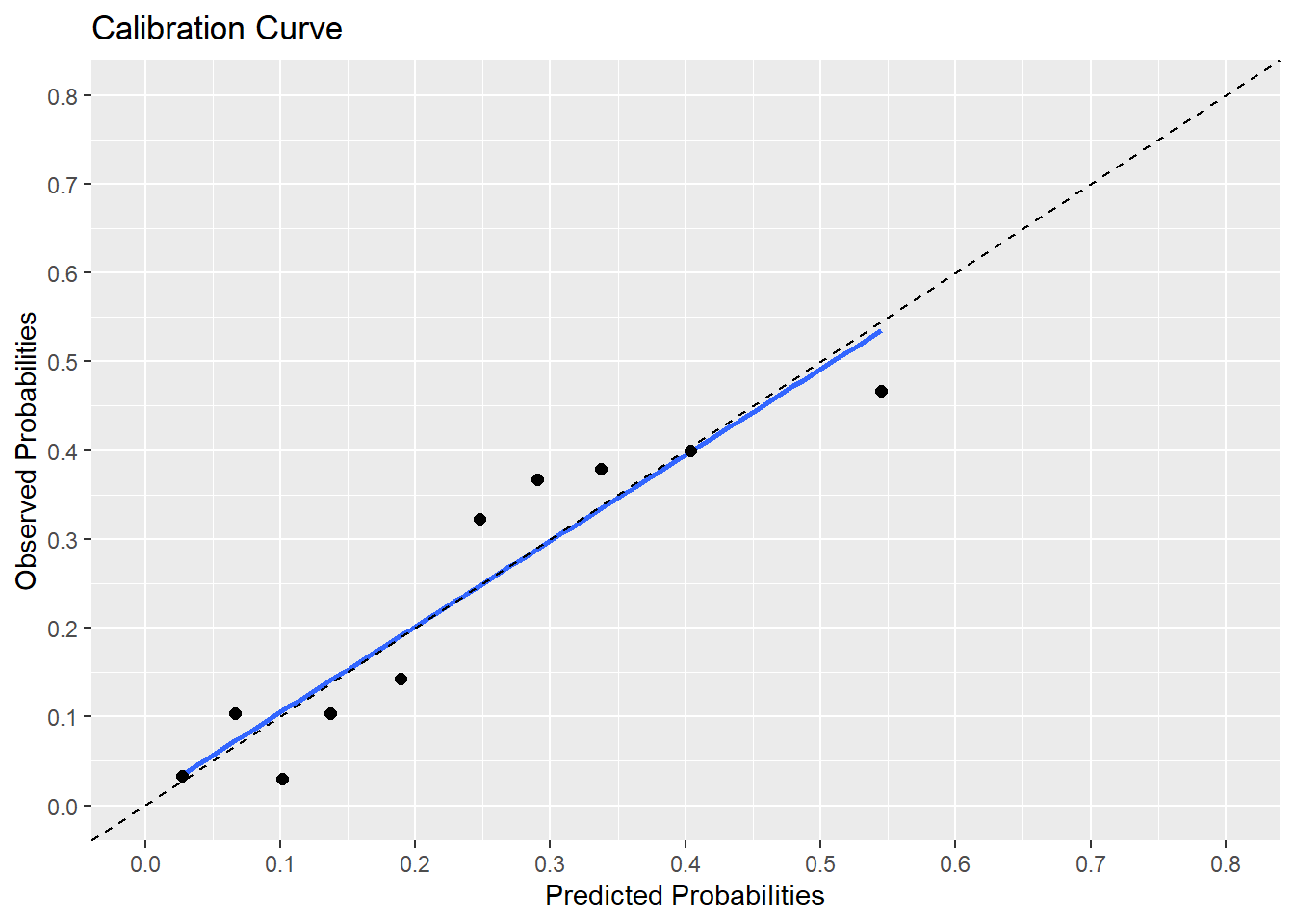
Hosmer and Lemeshow test
hoslem.test(fit.ext$y, pred.ext.recal)##
## Hosmer and Lemeshow goodness of fit (GOF) test
##
## data: fit.ext$y, pred.ext.recal
## X-squared = 5.9383, df = 8, p-value = 0.6541The Hosmer and Lemeshow test is not significant and the calibration curve looks as if the model calibrates well in the external dataset. This is incorrect and the result of working with calibrated predictions. As you may have noticed, these calibrated predictions do not influence the ROC curve and AUC.