Recalibration of the Cox model Baseline Hazard Function after Shrinkage
Generating sample survival data
I generate a small dataset with some example data that has no further meaning but is used to compare results. The dataset contains a time, status, continuous and dichotomous variable.
set.seed(8284)
n <- 15
x1 <- rnorm(n)
x2 <- rbinom(n, 1, 0.7)
X <- cbind(x1, x2)
colnames(X) <- c("x1", "x2")
beta_true <- c(0.8, -0.5)

h0 <- 0.1  # constant baseline hazard

# linear predictor and survival times
LP_true <- X %*% beta_true
T_event <- rexp(n, rate = as.numeric(h0 * exp(LP_true)))
C <- rexp(n, rate = 0.15)
time <- pmin(T_event, C)
status <- as.integer(T_event <= C)

dat <- data.frame(time = time, status = status, X)
print(dat)
## time status x1 x2
## 1 11.6452145 0 -1.15997331 1
## 2 11.9546509 1 0.24323493 0
## 3 6.5568061 0 -0.05651773 1
## 4 10.7845487 0 0.85035738 1
## 5 6.8575038 1 1.35094683 1
## 6 1.3656016 1 2.38539478 1
## 7 6.5143091 0 1.59643397 1
## 8 13.6411050 1 -0.37149123 1
## 9 0.3101726 0 0.48354893 0
## 10 5.4913030 1 -0.18398557 1
## 11 4.5790413 1 1.34070837 1
## 12 4.4963411 0 0.67235594 1
## 13 2.1050665 0 0.05044414 1
## 14 0.3567029 0 0.72108005 1
## 15 13.6965845 0 1.82171965 1Estimate the Cox model
We estimate the Cox model using the example dataset.
fit_orig <- coxph(Surv(time, status) ~ x1 + x2, x=TRUE, y=TRUE, data = dat)summary(fit_orig)## Call:
## coxph(formula = Surv(time, status) ~ x1 + x2, data = dat, x = TRUE,
## y = TRUE)
##
## n= 15, number of events= 6
##
## coef exp(coef) se(coef) z Pr(>|z|)
## x1 0.2732 1.3141 0.4490 0.608 0.543
## x2 -0.4508 0.6371 1.1957 -0.377 0.706
##
## exp(coef) exp(-coef) lower .95 upper .95
## x1 1.3141 0.761 0.54504 3.168
## x2 0.6371 1.570 0.06115 6.638
##
## Concordance= 0.649 (se = 0.159 )
## Likelihood ratio test= 0.46 on 2 df, p=0.8
## Wald test = 0.43 on 2 df, p=0.8
## Score (logrank) test = 0.44 on 2 df, p=0.8Calculate the linear predictor of the Cox model
First I provide the linear predictor values of the Cox model extracted from the model fit by using the predict function, followed by a manual calculation. Both provide the same result. These linear predictor values are relative values to the sample mean value (see the previous post “Prediction Modeling with the Cox model - all about the baseline hazard” for more details) and calculated as:
\[LP_{sample} = \sum fit_{mean}*\beta's\]
\[LP_{indiv} = \sum X_i*\beta's\]
\[\widehat{LP} = LP_{indiv} - LP{sample}\]
First, we extract the values from the predict function.
LP_hat <- predict(fit_orig, newdata = dat, type = "lp")
LP_hat
## 1 2 3 4 5 6
## -0.94513787 -0.11100825 -0.64371553 -0.39599154 -0.25924944 0.02332263
## 7 8 9 10 11 12
## -0.19219163 -0.72975438 -0.04536356 -0.67853493 -0.26204620 -0.44461481
## 13 14 15
## -0.61449759 -0.43130522 -0.13065210Manual calculation gives the same result. For the manual calculation we use the coefficients from the Cox model and the mean covariate values to calculate the sample reference value. For dichotomous values 0 is used as reference value.
coef(fit_orig)## x1 x2
## 0.2731622 -0.4508262fit_orig$means## x1 x2
## 0.6496171 0.0000000LP_indiv <- (0.2731622*dat$x1) + (-0.4508262*dat$x2)
LP_sample <- sum(c((0.2731622*0.6496171), (-0.4508262*0) ))
LP_manual <- LP_indiv-LP_sample
LP_manual## [1] -0.94513790 -0.11100825 -0.64371554 -0.39599154 -0.25924943 0.02332265
## [7] -0.19219162 -0.72975440 -0.04536355 -0.67853494 -0.26204619 -0.44461481
## [13] -0.61449760 -0.43130522 -0.13065209Shrink the coefficients and linear predictor of the Cox model
We can shrink the coefficients and linear predictor of the Cox model by using different methods. We show them here. We start by using a shrinkage factor of 1, so no effective shrinkage will be applied. We call the linear predictor lp_shrunk because later on we will use a shrinkage factor below 1 to effectively shrink the coefficients and subsequently recalibrate the baseline hazard. Now we use a shrinkage factor of 1, which makes that lp_shrunk is equal to LP_hat and LP_manual from the previous paragraph.
Indirectly Shrinking the LP by shrinking the coefficients first
We start by applying a shrinkage factor to the coefficients first.
In formula form, where \(s\) is the shrinkage factor:
\[\beta_{shrunk} = \beta_{orig}*s\]
\[LP_{sample \,shrunk} = \sum fit_{mean}*\beta_{shrunk}\]
\[LP_{indiv \,shrunk} = \sum X_i*\beta_{shrunk}\]
\[\widehat{LP_{shrunk}} = LP_{indiv \, shrunk} - LP_{sample \,shrunk}\]
s = 1 # s = shrinkage factor

coef_hat <- coef(fit_orig)
coef_shrunk <- coef_hat * s

lp_sample_shrunk <- sum((coef_shrunk) * fit_orig$means)
lp_indiv_shrunk <- as.vector(as.matrix(dat[, c("x1","x2")]) %*% (coef_shrunk))
lp_shrunk <- lp_indiv_shrunk - lp_sample_shrunk
lp_shrunk
## [1] -0.94513787 -0.11100825 -0.64371553 -0.39599154 -0.25924944 0.02332263
## [7] -0.19219163 -0.72975438 -0.04536356 -0.67853493 -0.26204620 -0.44461481
## [13] -0.61449759 -0.43130522 -0.13065210Directly Shrinking the LP
We apply a shrinkage factor directly to the linear predictor values.
In formula form:
\[\widehat{LP_{shrunk}} = \widehat{LP} * s\]
Both methods will provide the same result.
s = 1

lp_shrunk <- predict(fit_orig, newdata=dat, type="lp") * s
lp_shrunk
## 1 2 3 4 5 6
## -0.94513787 -0.11100825 -0.64371553 -0.39599154 -0.25924944 0.02332263
## 7 8 9 10 11 12
## -0.19219163 -0.72975438 -0.04536356 -0.67853493 -0.26204620 -0.44461481
## 13 14 15
## -0.61449759 -0.43130522 -0.13065210Offset of the Linear predictor
Now we are going to use the offset of the linear predictor in the Cox model to first evaluate what happens with the linear predictor values of that model. We start with an example where no shrinkage is applied (we use the same lp_shrunk as defined above, with a shrinkage factor s of 1). In the next paragraph we will see the effect of the offset model on the baseline hazard values.
fit_offset <- coxph(Surv(time, status) ~ offset(lp_shrunk), x=TRUE, y=TRUE, data = dat)fit_offset## Call: coxph(formula = Surv(time, status) ~ offset(lp_shrunk), data = dat,
## x = TRUE, y = TRUE)
##
## Null model
## log likelihood= -10.42071
## n= 15fit_offset$linear.predictors ## 1 2 3 4 5 6
## -0.94513787 -0.11100825 -0.64371553 -0.39599154 -0.25924944 0.02332263
## 7 8 9 10 11 12
## -0.19219163 -0.72975438 -0.04536356 -0.67853493 -0.26204620 -0.44461481
## 13 14 15
## -0.61449759 -0.43130522 -0.13065210The linear predictor values of the offset model are the same as the lp_shrunk values from the original Cox model. This is what we expect because we re-fit the same model.
The baseline hazard of the offset model
Now we compare the baseline hazard function values of the original Cox model fit and the model where we used the linear predictor lp_shrunk as an offset procedure. Be aware, we still use the linear predictor without shrinkage, so the results of the baseline hazard values should be the same between the fit of the original and offset Cox model.
We start by extracting the baseline hazard values of the original model.
bh_fit_orig <- basehaz(fit_orig, centered = TRUE)bh_fit_orig## hazard time
## 1 0.0000000 0.3101726
## 2 0.0000000 0.3567029
## 3 0.1120994 1.3656016
## 4 0.1120994 2.1050665
## 5 0.1120994 4.4963411
## 6 0.2610182 4.5790413
## 7 0.4292099 5.4913030
## 8 0.4292099 6.5143091
## 9 0.4292099 6.5568061
## 10 0.6738432 6.8575038
## 11 0.6738432 10.7845487
## 12 0.6738432 11.6452145
## 13 1.1174041 11.9546509
## 14 1.8529414 13.6411050
## 15 1.8529414 13.6965845Followed by the baseline hazard values of the offset model.
bh_fit_offset <- basehaz(fit_offset, centered = TRUE)bh_fit_offset## hazard time
## 1 0.00000000 0.3101726
## 2 0.00000000 0.3567029
## 3 0.07584336 1.3656016
## 4 0.07584336 2.1050665
## 5 0.07584336 4.4963411
## 6 0.17659765 4.5790413
## 7 0.29039150 5.4913030
## 8 0.29039150 6.5143091
## 9 0.29039150 6.5568061
## 10 0.45590362 6.8575038
## 11 0.45590362 10.7845487
## 12 0.45590362 11.6452145
## 13 0.75600463 11.9546509
## 14 1.25364875 13.6411050
## 15 1.25364875 13.6965845That is remarkable. We see now that they provide different results. Let’s see if we can find an answer by reading the help information of the basehaz function. We read there: “Offset terms can pose a particular challenge for the underlying code and are always re-centered; to override this use the newdata argument and include the offset as one of the variables.”
Let us focus on the following parts: “and are always recentered” and “use the newdata argument”. What does that mean? Let’s explore first what happens when we re-center the offset term”, followed by “use the newdata argument”.
Re-centering the offset term
We use the manual Breslow formula calculation (see the previous post “Prediction Modeling with the Cox model - all about the baseline hazard” for more details) to see what happens with the calculation of the baseline hazard when we re-center the linear predictor of the offset model, i.e. lp_shrunk by subtracting the mean value of lp_shrunk from lp_shrunk itself. Remember, lp_shrunk, the linear predictor of the offset model is still the same as the original model here because the shrinkage factor was 1 in the calculation of lp_shrunk.
mean_lp_shrunk <- mean(lp_shrunk)

breslow_est <- function(time, status, X, B){
  data <-
    data.frame(time, status, X)
  data <-
    data[order(data$time), ]
  t   <-
    unique(data$time)
  k    <-
    length(t)
  h    <-
    rep(0,k)

  for(i in 1:k) {
    LP_sample <- sum(fit_orig$means * coef(fit_orig))
    LP_indiv <- (data.matrix(data[,-c(1:2)]) %*% B)
    lp_shrunk <- LP_indiv - LP_sample

    lp <- (lp_shrunk-mean_lp_shrunk)[data$time>=t[i]] # re-centering the offset term

    risk <- exp(lp)
    h[i] <- sum(data$status[data$time==t[i]]) / sum(risk)
  }

  res <- cumsum(h)
  return(res)
}

H0 <- breslow_est(time=dat$time, status=dat$status, X=fit_orig$x, B=coef(fit_orig))
H0
## [1] 0.00000000 0.00000000 0.07584336 0.07584336 0.07584336 0.17659765
## [7] 0.29039150 0.29039150 0.29039150 0.45590362 0.45590362 0.45590362
## [13] 0.75600463 1.25364875 1.25364875This gives indeed the same INCORRECT results as in the previous paragraph where we used the basehaz function for the offset model, which was.
bh_fit_offset <- basehaz(fit_offset, centered = TRUE)bh_fit_offset## hazard time
## 1 0.00000000 0.3101726
## 2 0.00000000 0.3567029
## 3 0.07584336 1.3656016
## 4 0.07584336 2.1050665
## 5 0.07584336 4.4963411
## 6 0.17659765 4.5790413
## 7 0.29039150 5.4913030
## 8 0.29039150 6.5143091
## 9 0.29039150 6.5568061
## 10 0.45590362 6.8575038
## 11 0.45590362 10.7845487
## 12 0.45590362 11.6452145
## 13 0.75600463 11.9546509
## 14 1.25364875 13.6411050
## 15 1.25364875 13.6965845In the help description of the basehaz function you can read at the centered option “if FALSE return a prediction for all covariates equal to zero”. You could think that you get the same result when you use the basehaz function and choose for centered is FALSE. Let’s try that also.
bh_offset <- basehaz(fit_offset, centered = FALSE)bh_offset## hazard time
## 1 0.00000000 0.3101726
## 2 0.00000000 0.3567029
## 3 0.07584336 1.3656016
## 4 0.07584336 2.1050665
## 5 0.07584336 4.4963411
## 6 0.17659765 4.5790413
## 7 0.29039150 5.4913030
## 8 0.29039150 6.5143091
## 9 0.29039150 6.5568061
## 10 0.45590362 6.8575038
## 11 0.45590362 10.7845487
## 12 0.45590362 11.6452145
## 13 0.75600463 11.9546509
## 14 1.25364875 13.6411050
## 15 1.25364875 13.6965845We see however, that we still provide the same INCORRECT result. This also means that the basehaz function is insensitive for the centered option after fitting the offset model.
Use the newdata argument
Let’s see what happens when we use the newdata option in the basehaz function. It is described in the help file of that function that the centered option is ignored if the newdata argument is used. The question is now, what kind of value for lp_shrunk do we need for the newdata argument.
It seems that we have to use the value 0 to prevent re-centering. Let’s see what happens when we do that. We set the value for lp_shrunk at 0.
mean(lp_shrunk)## [1] -0.390716bh_offset <- basehaz(fit_offset, newdata=data.frame(lp_shrunk=0))bh_offset## hazard time
## 1 0.0000000 0.3101726
## 2 0.0000000 0.3567029
## 3 0.1120994 1.3656016
## 4 0.1120994 2.1050665
## 5 0.1120994 4.4963411
## 6 0.2610182 4.5790413
## 7 0.4292099 5.4913030
## 8 0.4292099 6.5143091
## 9 0.4292099 6.5568061
## 10 0.6738432 6.8575038
## 11 0.6738432 10.7845487
## 12 0.6738432 11.6452145
## 13 1.1174041 11.9546509
## 14 1.8529414 13.6411050
## 15 1.8529414 13.6965845now we get the same cumulative hazard values as the original model when we had used centered is TRUE. This is a good starting point to apply shrinkage of the coefficients and linear predictor and subsequently adjust the baseline hazard function.
Shrinking the Cox model and adjusting the baseline hazard
We start by shrinking the Cox model and use a shrinkage factor of 0.7.
s = 0.7

lp_shrunk_correct <- predict(fit_orig, newdata=dat, type="lp") * s
lp_shrunk_correct
## 1 2 3 4 5 6
## -0.66159651 -0.07770578 -0.45060087 -0.27719408 -0.18147461 0.01632584
## 7 8 9 10 11 12
## -0.13453414 -0.51082807 -0.03175449 -0.47497445 -0.18343234 -0.31123037
## 13 14 15
## -0.43014832 -0.30191366 -0.09145647Offset the Linear predictor
Now we use the shrunken linear predictor as an offset in the Cox model.
fit_offset <- coxph(Surv(time, status) ~ offset(lp_shrunk_correct), x=TRUE, y=TRUE, data = dat)Recalibrate the baseline hazard function
Finally we use the basehaz function to recalibrate the baseline hazard values (and prevent the re-centering of lp_shrunk_correct).
bh_offset_correct <- basehaz(fit_offset, newdata=data.frame(lp_shrunk_correct=0))bh_offset_correct## hazard time
## 1 0.0000000 0.3101726
## 2 0.0000000 0.3567029
## 3 0.1008990 1.3656016
## 4 0.1008990 2.1050665
## 5 0.1008990 4.4963411
## 6 0.2340284 4.5790413
## 7 0.3837496 5.4913030
## 8 0.3837496 6.5143091
## 9 0.3837496 6.5568061
## 10 0.6037324 6.8575038
## 11 0.6037324 10.7845487
## 12 0.6037324 11.6452145
## 13 1.0139323 11.9546509
## 14 1.6750458 13.6411050
## 15 1.6750458 13.6965845With these recalibrated baseline hazard values we can calculate and plot cumulative hazard and survival curves.
Cumulative Hazard and Survival curves before and after shrinkage
Now we can compare the cumulative hazard and survival curves before and after shrinkage of the Cox model and adjusting the baseline hazard.
Before shrinkage (original model)
fit_orig <- coxph(Surv(time, status) ~ x1 + x2,
                  x=TRUE, y=TRUE, data = dat)

model_surv <- survfit(fit_orig)

df_surv_orig <- data.frame(time=model_surv$time, surv=model_surv$surv, hazard=model_surv$cumhaz)
df_surv_orig
## time surv hazard
## 1 0.3101726 1.0000000 0.0000000
## 2 0.3567029 1.0000000 0.0000000
## 3 1.3656016 0.8939554 0.1120994
## 4 2.1050665 0.8939554 0.1120994
## 5 4.4963411 0.8939554 0.1120994
## 6 4.5790413 0.7702669 0.2610182
## 7 5.4913030 0.6510233 0.4292099
## 8 6.5143091 0.6510233 0.4292099
## 9 6.5568061 0.6510233 0.4292099
## 10 6.8575038 0.5097458 0.6738432
## 11 10.7845487 0.5097458 0.6738432
## 12 11.6452145 0.5097458 0.6738432
## 13 11.9546509 0.3271279 1.1174041
## 14 13.6411050 0.1567753 1.8529414
## 15 13.6965845 0.1567753 1.8529414library(ggplot2)
# Create the plot
ggplot(df_surv_orig, aes(x = time, y = hazard)) +
geom_step() +
labs(title = "Cumulative Hazard from Cox Model",
x = "Time",
y = "Cumulative Hazard") 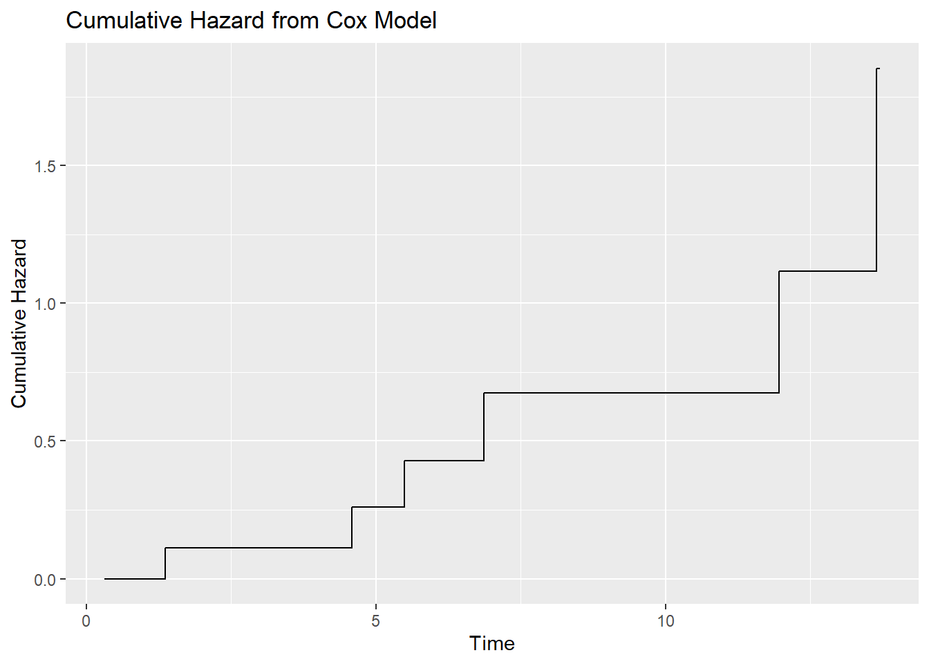
ggplot(df_surv_orig, aes(x = time, y = surv)) +
  geom_step() +
  labs(title = "Survival Curve from Cox Model",
       x = "Time",
       y = "Survival Probability") +
  theme_minimal() +
  ylim(0, 1)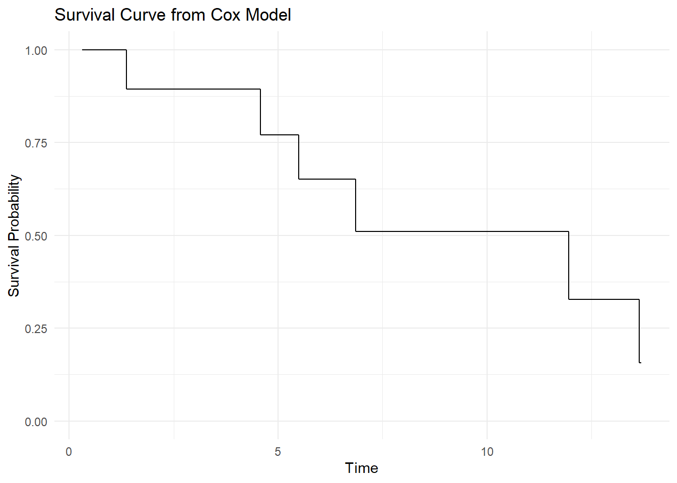
After shrinkage (recalibrated model)
fit_offset <- coxph(Surv(time, status) ~ offset(lp_shrunk_correct), x=TRUE, y=TRUE, data = dat)

model_surv_offset <- survfit(fit_offset, newdata=data.frame(lp_shrunk_correct=0))

df_surv_total <- data.frame(time=model_surv_offset$time,
                            df_surv_orig,
                            surv_shrink=model_surv_offset$surv,
                            hazard_shrink=model_surv_offset$cumhaz)

df_surv_total[, -2] # exclude 1 time variable
## time surv hazard surv_shrink hazard_shrink
## 1 0.3101726 1.0000000 0.0000000 1.0000000 0.0000000
## 2 0.3567029 1.0000000 0.0000000 1.0000000 0.0000000
## 3 1.3656016 0.8939554 0.1120994 0.9040244 0.1008990
## 4 2.1050665 0.8939554 0.1120994 0.9040244 0.1008990
## 5 4.4963411 0.8939554 0.1120994 0.9040244 0.1008990
## 6 4.5790413 0.7702669 0.2610182 0.7913393 0.2340284
## 7 5.4913030 0.6510233 0.4292099 0.6813020 0.3837496
## 8 6.5143091 0.6510233 0.4292099 0.6813020 0.3837496
## 9 6.5568061 0.6510233 0.4292099 0.6813020 0.3837496
## 10 6.8575038 0.5097458 0.6738432 0.5467670 0.6037324
## 11 10.7845487 0.5097458 0.6738432 0.5467670 0.6037324
## 12 11.6452145 0.5097458 0.6738432 0.5467670 0.6037324
## 13 11.9546509 0.3271279 1.1174041 0.3627896 1.0139323
## 14 13.6411050 0.1567753 1.8529414 0.1872996 1.6750458
## 15 13.6965845 0.1567753 1.8529414 0.1872996 1.6750458library(tidyr)
df_long <- df_surv_total %>%
pivot_longer(
cols = c(surv,
surv_shrink,
hazard,
hazard_shrink),
names_to = "group",
values_to = "probability"
)
library(dplyr)
df_long_cumhaz <- df_long %>% filter(group == "hazard" | group == "hazard_shrink")
## Hazard curves
ggplot(df_long_cumhaz, aes(x = time, y = probability, color = group)) +
geom_step(linewidth = 1.2) +
scale_y_continuous(name = "Survival Probability") +
scale_x_continuous(name = "Time") +
labs(
title = "Cumulative Hazard Curves",
subtitle = "Plotting Cumulative Hazard",
color = "Group"
) +
theme_classic() 
df_long_surv <- df_long %>% filter(group == "surv" | group == "surv_shrink")
## Survival curves
ggplot(df_long_surv, aes(x = time, y = probability, color = group)) +
  geom_step(linewidth = 1.2) +
  scale_y_continuous(limits = c(0, 1), name = "Survival Probability") +
  scale_x_continuous(name = "Time") +
  labs(
    title = "Survival Curves ",
    subtitle = "Plotting survival probabilities",
    color = "Group"
  ) +
theme_classic() 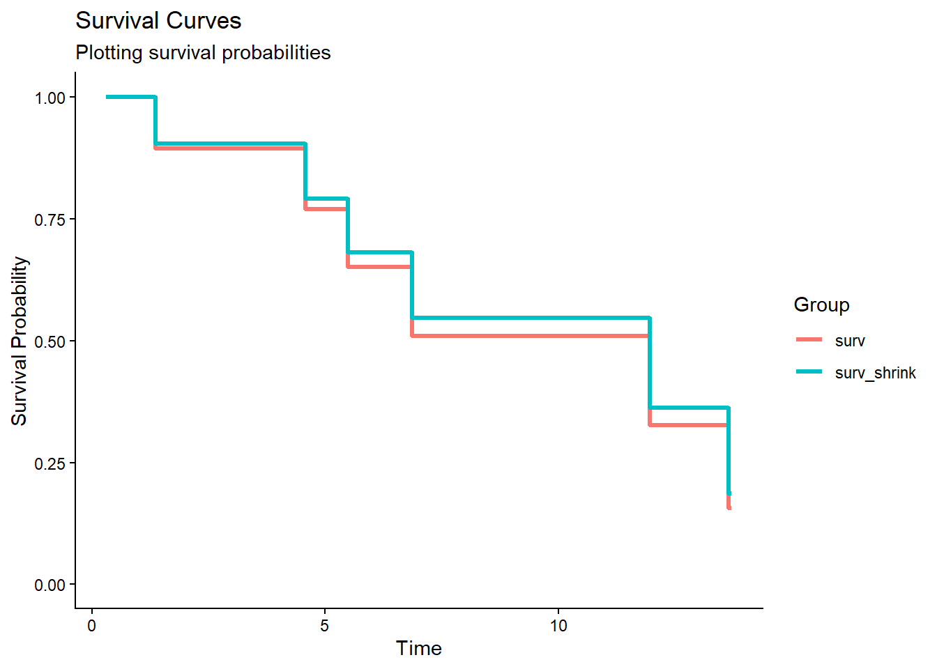
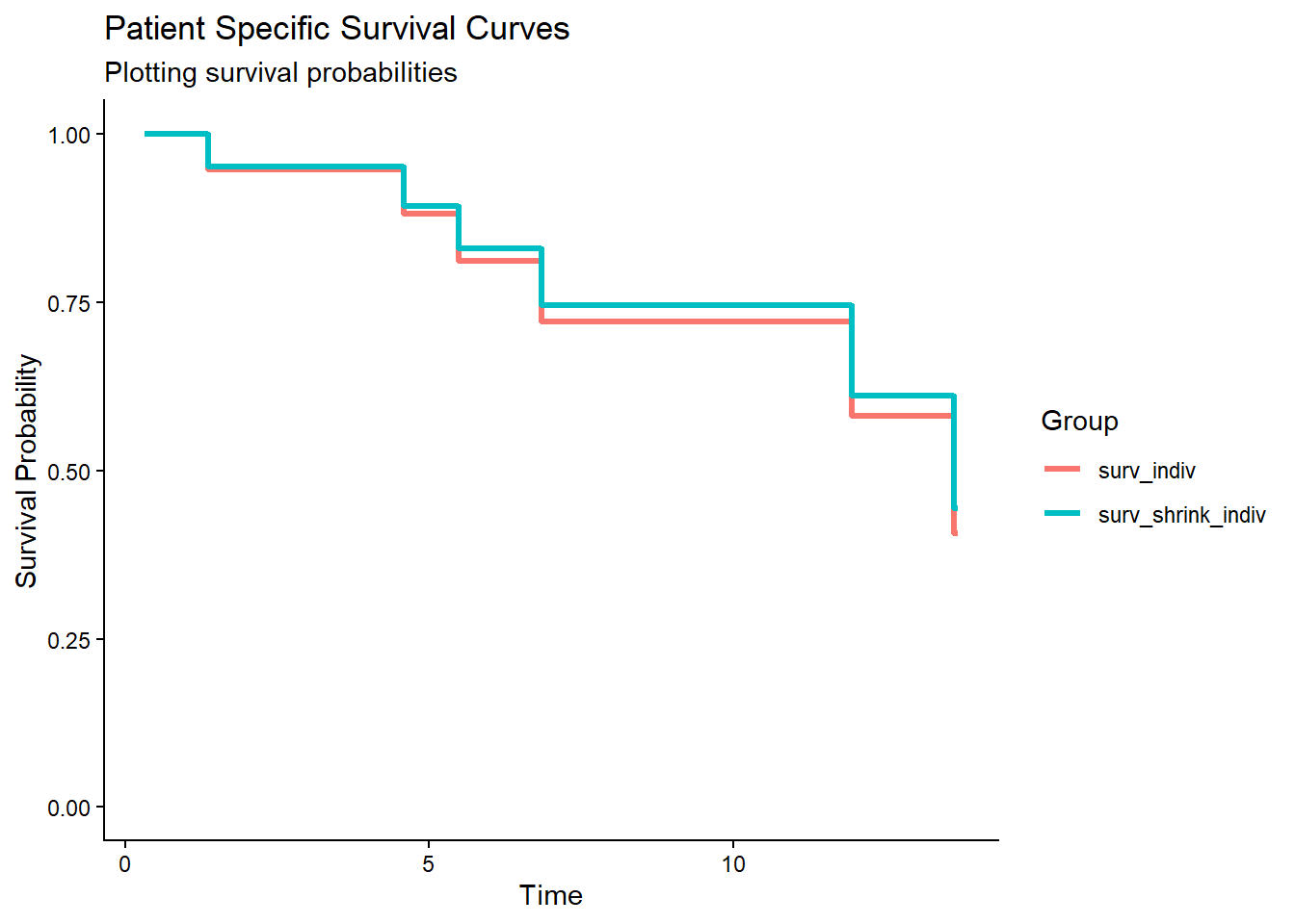
Patient Specific Survival Curves
We can now also generate patient specific survival curves for each patient covariate pattern. We use here a patient with the values -2 and 0 for the variables x1 and x2 respectively. We compare again the survival curves before and after shrinkage of the Cox model.
LP_indiv <- predict(fit_orig, newdata = data.frame(x1 = -2,
                                             x2 = 0), type="lp")
LP_indiv # linear predictor value of specific values of individual patient (values are centered)
## 1
## -0.7237752H0 <- basehaz(fit_orig, centered=TRUE) # baseline hazard of original model.
cumhaz_indiv <- H0[, 1]*exp(LP_indiv) # cumulative hazard of individual patient before shrinkage
surv_indiv <- exp(-cumhaz_indiv) # survival probability of individual patient before shrinkage
df_surv_indiv <- data.frame(time=model_surv$time, surv=surv_indiv)
H0_offset <- basehaz(fit_offset, newdata=data.frame(lp_shrunk_correct=0)) # baseline hazard of shrunken model
cumhaz_offset <- H0_offset[, 1]*exp(LP_indiv) # cumulative hazard of individual patient from shrunken model
surv_indiv_offset <- exp(-cumhaz_offset) # survival probability of individual patient of shrunken model
df_surv_total_indiv <- data.frame(time=model_surv_offset$time,
surv_indiv = surv_indiv,
surv_shrink_indiv=surv_indiv_offset)
df_surv_total_indiv## time surv_indiv surv_shrink_indiv
## 1 0.3101726 1.0000000 1.0000000
## 2 0.3567029 1.0000000 1.0000000
## 3 1.3656016 0.9470920 0.9522499
## 4 2.1050665 0.9470920 0.9522499
## 5 4.4963411 0.9470920 0.9522499
## 6 4.5790413 0.8811103 0.8927179
## 7 5.4913030 0.8121001 0.8302012
## 8 6.5143091 0.8121001 0.8302012
## 9 6.5568061 0.8121001 0.8302012
## 10 6.8575038 0.7212577 0.7462006
## 11 10.7845487 0.7212577 0.7462006
## 12 11.6452145 0.7212577 0.7462006
## 13 11.9546509 0.5816714 0.6116016
## 14 13.6411050 0.4071698 0.4438538
## 15 13.6965845 0.4071698 0.4438538df_long_indiv <- df_surv_total_indiv %>%
pivot_longer(
cols = c(surv_indiv,
surv_shrink_indiv),
names_to = "group",
values_to = "probability"
)
ggplot(df_long_indiv, aes(x = time, y = probability, color = group)) +
geom_step(linewidth = 1.2) +
scale_y_continuous(limits = c(0, 1), name = "Survival Probability") +
scale_x_continuous(name = "Time") +
labs(
title = "Patient Specific Survival Curves ",
subtitle = "Plotting survival probabilities",
color = "Group"
) +
theme_classic()